
Tutorial - Simple Calculations With Units
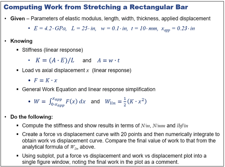
This tutorial demonstrates how to perform several units-oriented calculations with Kornucopia and MATLAB. The example demonstrated involves the analytical calculation of the work generate by stretching an elastic rectangular bar.
Contents
Overview
%{
Key concepts and features demonstrated include:
 o Working with variables and units, and also other Props of
   variables of type k_units.
 o Utilizing several other Kornucopia and MATLAB function to further
   process and evaluate/plot data.

Tips:
 o Consider running the example "By Section". It will help you walk
   through the example and its results.
%}
Set-up
%{
This section makes a few initial settings for the example.

Additional Details:
The settings below include:
 o Popup asking to clean MATLAB session before start of example.
 o Saving your current settings for all ADV settings, Units
   Preference, and MATLAB format. These will be reset to their
   respective values at the end of the example.
 o Define a handy "adv" variable so that we can later use it to
   quickly access any Kornucopia function's ADV options with ease.
 o The comment #ok<*NOPTS> at the end of this section suppresses a
   MATLAB warning about not including semicolon at end of statements.
     - While we would normally use semicolons at end of MATLAB
       statements, several of the variable definitions later do not so
       that they conveniently echo to the MATLAB window.
%}

k_cleanup({'BEFORE starting the example:'; ' '});
origSettings = k_exampleSetup();
adv = k_adv();
disp(' ')

%#ok<*NOPTS>
Problem description
%{
The image that will appear in this section describes the problem.
You may elect to keep it open so you can see what we are trying to
accomplish in the problem.
%}

dataDir = k_examplesDir('data');
imageName = 'workFromStretchingBar.png';
fullImageName = fullfile(dataDir, 'media', imageName);

k_picDisplay(fullImageName, 'center');
Specifying the inputs
%{
Below we define the input parameters for the problem, including
assigning units to them via simple multiplication with the units
variables we defined above. Kornucopia will automatically handle the
fact that we are supplying inputs in mixed units.

Additional Details:
 o In this example, we used unitsVariables to define our variables
   with units, like the variable of length, L. We could also have
   used the k_units function instead of unitsVariables as in
      L = k_units(25, 'in')
   If it was done this way, then L would display its results in
   the units of inches because no math has been done on L yet, only
   its creation via k_units.
 o Since our unitsPreference is set to 'mm_N_s', this means that when
   any math is done, the results will be converted as needed to return
   results in this unitPreference. Note that making a statement like
      L = 25*in
   is actually a multiplication of "25" and "in", thus we are doing
   math, and hence the result returned is converted into "mm" since
   that is what our unitsPreference requests.
 o We also create a well-documented summary variable that will be
   placed on the final plots later.
%}

% Setting a specific Units Preference for this example.
k_unitsPreferenceActivate('mm_N_s');

% Defining some "unitsVariables" makes it easily apply units to other
% values or variables by simple multiplication.
k_unitsVariables('mm, in, GPa, J')

% Given the following parameters:
E = 4.2*GPa
L = 25*in
w = 0.1*in
t = 10*mm
xApp = 0.23*in

% Define a summary variable to put on plots later
inputs = [E, L, w, t, xApp];
inputs.Props.ColNames = 'E, L, w, t, xApp';
inputs.Props.Description = 'Input parameters';

inputsOrigUnits = inputs.convert('GPa, in, in, mm, in');
inputsOrigUnits.Props.Description = 'Inputs in original units';

% Echo the summary to the MATLAB command window.
disp(' ')
display(inputs)
display(inputsOrigUnits)
Units Preference now activated: 'mm_N_s'

E = 4200*MPa


L = 635.0*mm


w = 2.540*mm


t = 10.00*mm


xApp = 5.842*mm


inputs =
    Input parameters
    ================
      E        L        w        t      xApp
    [MPa]    [mm]     [mm]     [mm]     [mm]
    _____    _____    _____    _____    _____
     4200    635.0    2.540    10.00    5.842


inputsOrigUnits =
    Inputs in original units
    ========================
      E        L        w         t       xApp
    [GPa]    [in]      [in]     [mm]      [in]
    _____    _____    ______    _____    ______
    4.200    25.00    0.1000    10.00    0.2300
Calculate required results
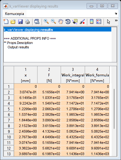
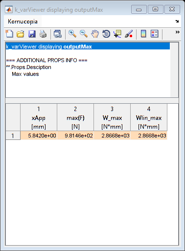
%{
Below we calculate the required results from the inputs.

Additional Details:
 o For calculating the load and work as a function of displacement, we
   need multiple values of x. We use the k_vectorByPoints function to
   easily create a column vector of points.
    - We could also have issued a command like
      x = [0:1:nPoints]' * xApp; % note ' is transpose
    - It is NOT advised to do 1 by nPoints row vectors in Kornucopia
      as this is very inefficient since it forces Kornucopia to keep
      track of a large number of units, one per column. Bottom line,
      Kornucopia is best used with data stored column-wise.
 o To help use keep track and for nicely and automatically formatted
   output later, we apply a few Props to some of the variables.
   Applying Props such as ColNames or Descriptions is optional, but
   often it is very helpful.
 o You will notice a few warnings echo to the screen stating:
      "... the output result did NOT inherit any of the "Props" from
       the input argument(s)."
   This warning occurred when we calculated F = K*x and when we did
   Wlin = 0.5*(K * (x .^2)).
   The warning in these cases can be ignored, but to learn more about
   why the warning was issued, click on the warning's "learn more"
   link.
%}

% Calculate the cross-sectional area of bar and then its linear stiff
A = w*t
K = (A*E)/L

% Showing the stiffness in some other requested units
disp(K.convert('N/m'))
disp(K.convert('lbf/in'))

% Define a vector of displacements to compute the force and work over
nPoints = 20
x = k_vectorByPoints(0, 1, nPoints)*xApp;
x.Props.ColNames = 'Displacement'

F = K*x;
F.Props.ColNames = 'Force';

% Compute work by integration and then using the analytical formula
W = k_integrate(x,F); % We ignore the Initial Condition which is zero
W.Props.ColNames = 'Work_integral';
W_max = W(end,1); % the last value is the max.

Wlin = 0.5*(K * (x .^2));
Wlin.Props.ColNames = 'Work_formula';
Wlin_max = max(Wlin);  % This is another way to get max value

% Create some summary variables
results = [x, F, W, Wlin];
results.Props.ColNames = 'x, F, Work_integral, Work_formula';
results.Props.Description = 'Output results';

k_varViewer(results);

outputMax = [xApp, max(F), W_max, Wlin_max];
outputMax.Props.ColNames = 'xApp, max(F), W_max, Wlin_max';
outputMax.Props.Description = 'Max values';

% Show the max values in different units.
display(outputMax)
display(outputMax.convert('m, N, N*m, N*m'))
display(outputMax.convert('in, lbf, lbf*in, lbf*in'))
A = 25.40*mm^2


K = 168.0*N/mm

    1.680e+05*N/m

    959.3*lbf/in


nPoints =

    20


x =
    Displacement
        [mm]
    ____________
        0.000
       0.3075
       0.6149
       0.9224
        1.230
        1.537
        1.845
        2.152

    ... 12 rows not shown.
        See "n" rows via k_set('dispBrief', n).

outputMax =
    Max values
    ==========
    xApp     max(F)    W_max     Wlin_max
    [mm]      [N]      [N*mm]     [N*mm]
    _____    ______    ______    ________
    5.842     981.5     2867       2867


 =
    Max values
    ==========
      xApp      max(F)    W_max    Wlin_max
      [m]        [N]      [N*m]     [N*m]
    ________    ______    _____    ________
    0.005842     981.5    2.867      2.867


 =
    Max values
    ==========
     xApp     max(F)     W_max      Wlin_max
     [in]     [lbf]     [lbf*in]    [lbf*in]
    ______    ______    ________    ________
    0.2300     220.6      25.37       25.37
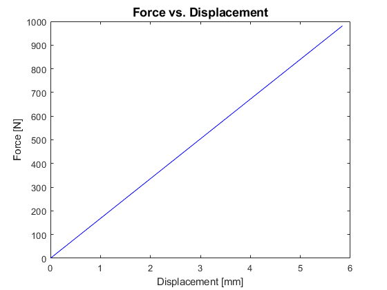
Simple plotting of the data
%{
In this section we just make two very simple plots of the results,
doing nothing fancy.

Additional Details:
 o You will notice that the two figures are on top of each other, and
   both are under the summary info of the outputMax.
 o Also notice that the legend in the work plot is "wimpy" and not
   all that helpful. Also you cannot tell the two curves from each
   other as they are on top of each other.
 o The legend is not located in the greatest location.
 o The summary info is in separate window via k_varViewer.
%}

figure('name', 'Force Vs Disp')
k_plot(x, F)

figure('name', 'Work Vs Disp')
k_plot(x, results('Work_integral, Work_formula'))

k_varViewer(outputMax);

msg = {'Note there are 3 figures stacked on top of each other.';...
       'Under the k_varViewer figure window is the plot of work,';...
       'and under that plot is the plot of force vs disp.'; ...
       ' '; 'This is the default behavior of MATLAB figures'; ...
       ' '; 'The next section shows how subplot helps with this.'};
warndlg(msg)

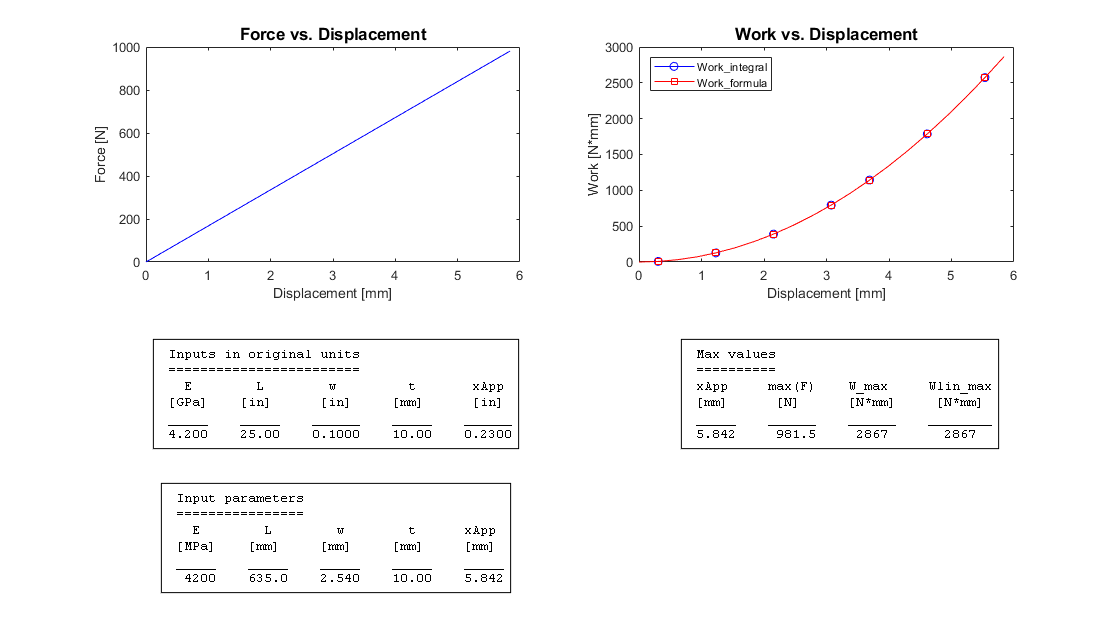
Fancy plotting of the results
%{
Below we create a final plot that summarizes the results.

Additional Details:
 o We use several ADV options along with subplot to achieve this
   well-formatted output.
 o The legentText option is used to apply further control of where the
   k_plot function pulls the text to fill the legend.
 o We turn on markerSymbols, pointing them to a Kornucopia list of
   markers. Also, we use an ADV to place a total of 7 markers along a
   curve. By default, Kornucopia will "jitter" the markers across
   multiple curves so that they do not tend to pile on top of each
   other. You can use additional ADV options to control many of these
   behaviors.
 o Lastly, we use k_displayOnFigure to have a nice presentation of
   the summary info on the figure too.
%}

figH = figure('name', 'Final Results', ...
    'position', k_figZoom(2, 1.5));

% Plot the force vs displacement
subplot(2,2,1)
k_plot(x, F)

% Plot the work vs displacement
subplot(2,2,2)
k_plot(x, results('Work_integral, Work_formula'), ...
    adv.k_plot.legendText.yColNames, ...
    'legendLocation', 'NorthWest', ...
    adv.k_plot.markerSymbols.list, ...
    adv.k_plot.markerOccurrence.USERinput2, {'total', 7})

% Displaying summary tables.
% We use the 'parent' ADV option to tell the software to on what
% parent object to place the information.

k_displayOnFigure(0.3, 0.45, inputsOrigUnits, ...
    'parent', figH, ...
    'box', 'on', ...
    'alignVert', 'top')

k_displayOnFigure(0.3, 0.07, inputs, ...
    'parent', figH, ...
    'box', 'on', ...
    'alignVert', 'bottom')


k_displayOnFigure(0.75, 0.45, outputMax, ...
    'parent', figH, ...
    'box', 'on', ...
    'alignVert', 'top')
End of example & optional clean-up
%{
Additional Details:
This section does the following:
 o Resets any changed preferences, such as Units Preferences and
   default ADV values back to their state prior to the example.
 o Resets the MATLAB format setting back to its original state prior
   to the example.
 o Opens an interactive dialog to offer the option of cleaning-up the
   MATLAB workspace.
%}

k_exampleSetup(origSettings);
Units Preference now activated: 'ShockVib_mm_ms_G'